Decision Trees and an introduction to Supervised Learning
In this section, the applications of decision trees will be discussed and its implementation demonstarted.
The first example will be of Record data in R with an additional implementation of Random Forest. The second example will be of text data in Python.
Concepts and Considerations
Decision Trees are the first method of suprevised learning that will be disucess. As such it is a good place to introduce the topic of supervised learning.
All prior demonstrations have been examples of unsupervised learning methods. The difference between supervised and unsupervised learning methods
is that
unsupervised learning tasks are performed on data that either do not have labeled data and or the labeled data is purposefully stripped from the data.
In supervised learning and specifically in classification, the goal is to predict the labeled data, where as in unsupervised methods such as clustering the goal is to,
in a simplified sense, find labels.
Record Data in R
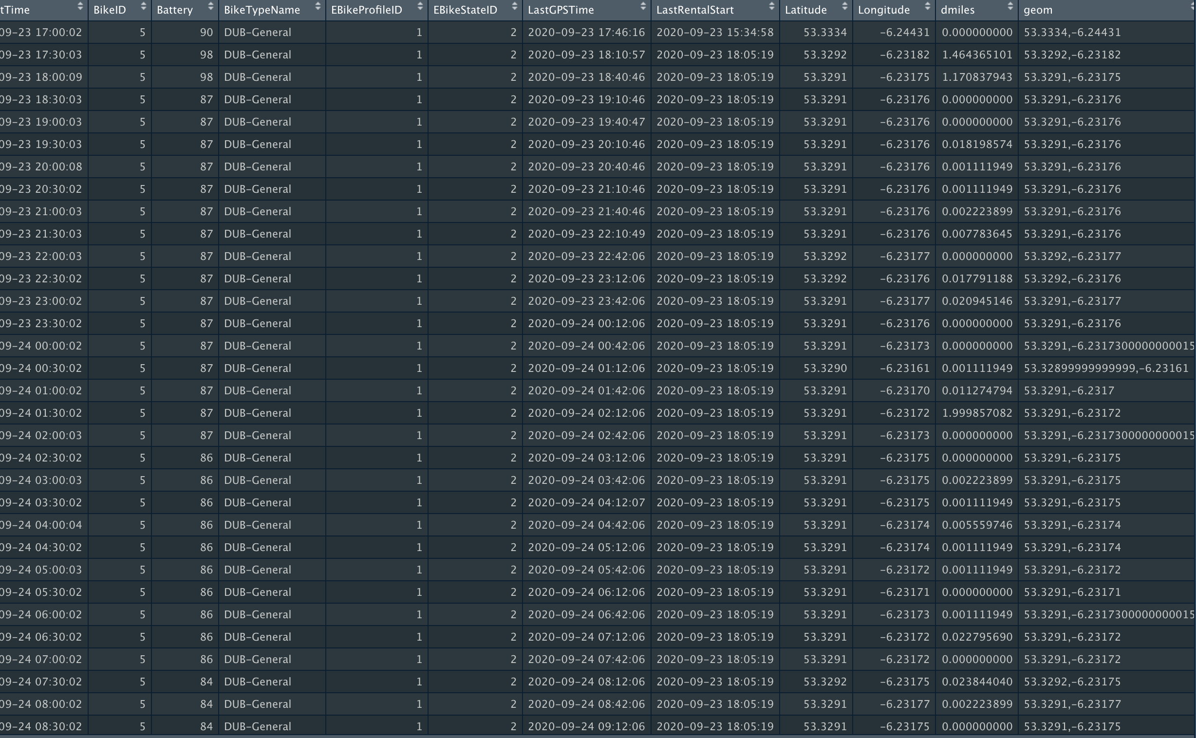
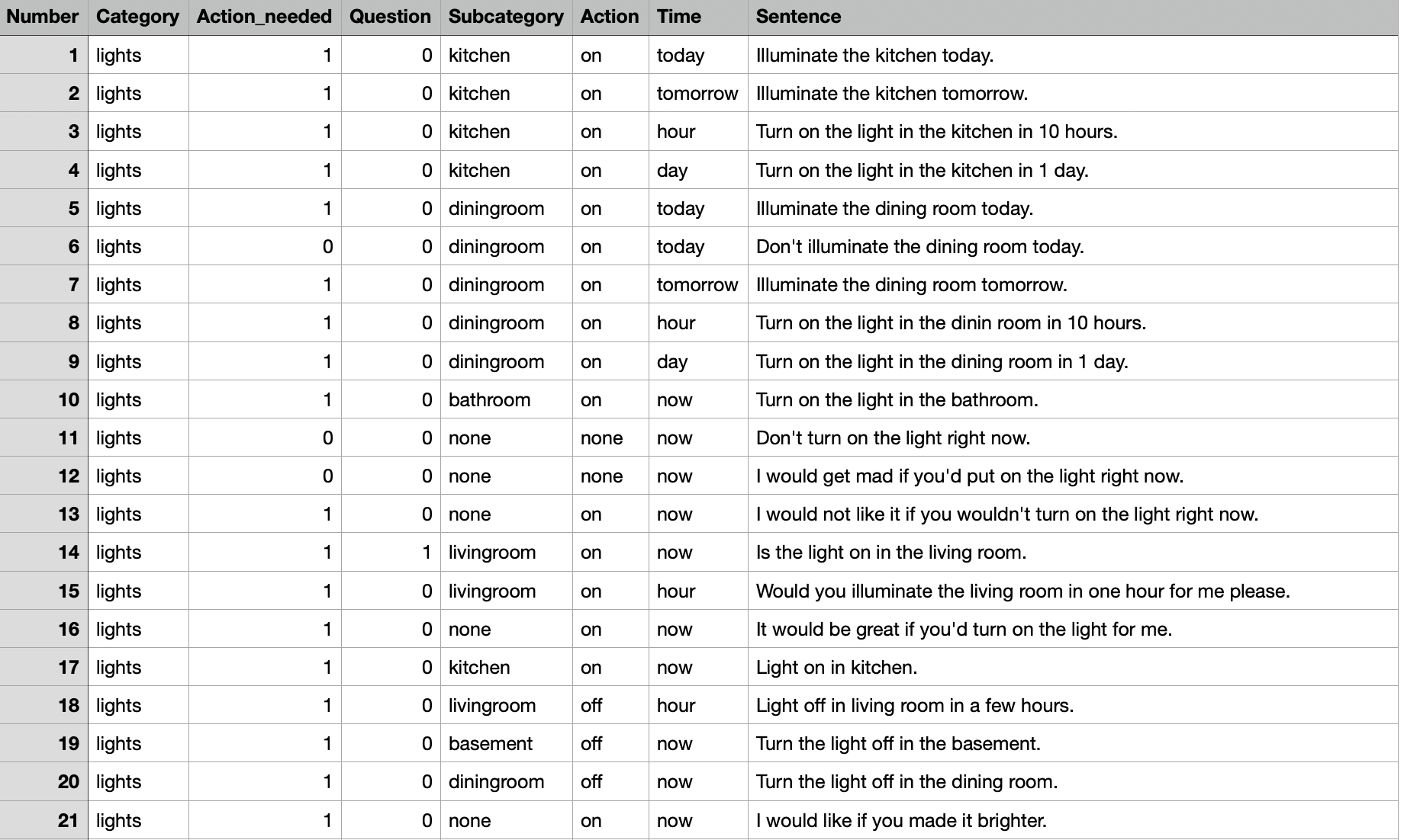
raw data
code

Data Cleaning:
For the Record data demonstration, the smartbikes data set will be used. The aim of this section is see if we can
predict the battery percentage of a bike, by providing other information.However, predicting the exact battery
percentage would be impossible since it is not an accurate lable. In order to over come this obstacle, the
Battery varibale was split into two groups, less than %50 and more than %50 (Discretization).
The new attribute titled "Battery.label" will be the label for our model.
Additionally, the variables BikeTypeName, EBikeStateID, weekday_int have been changed to type factor (categorical).
Data Visualizations:
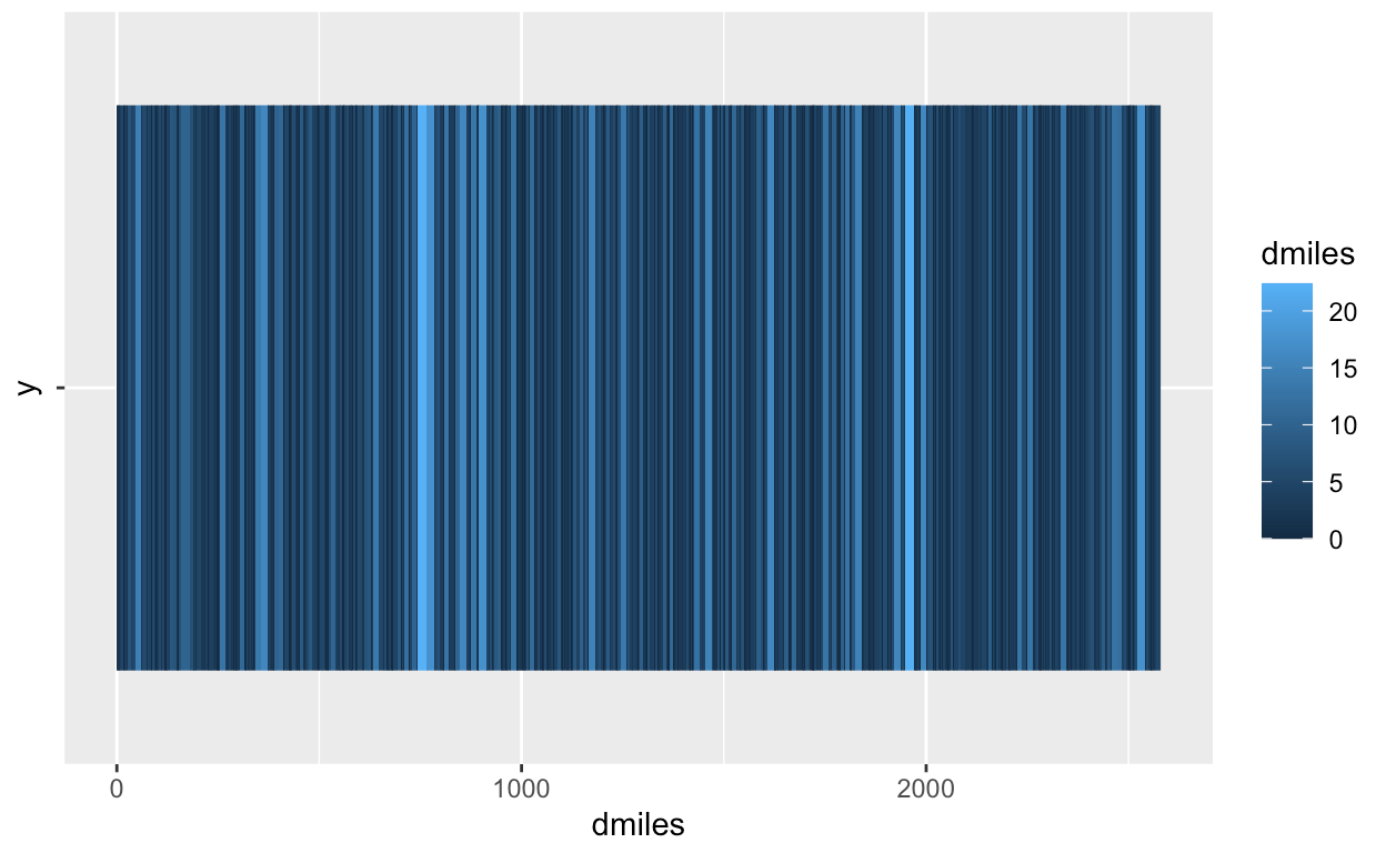
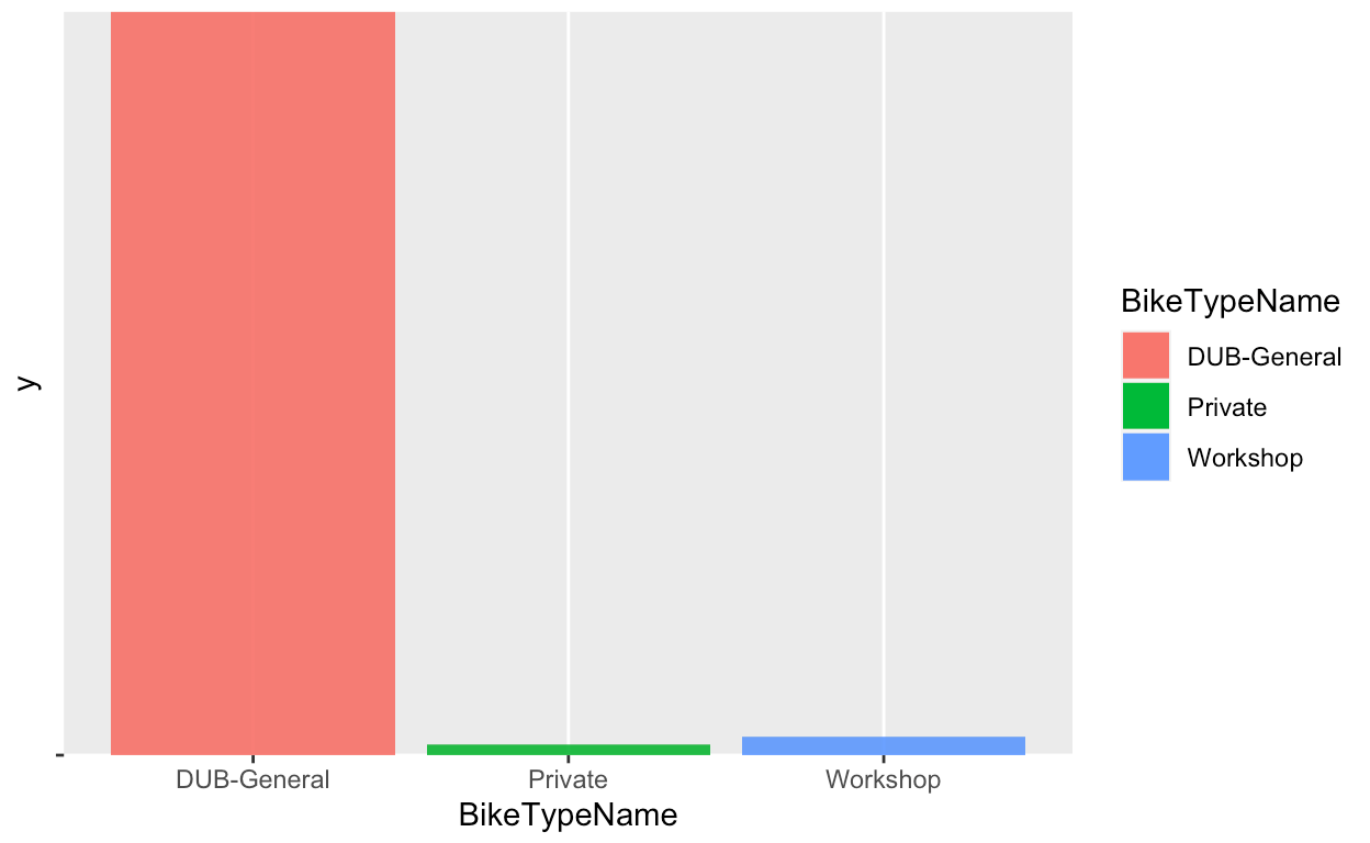
After the data cleaning process, a number of visualizations were created in order
better understand the datas statistical properties.


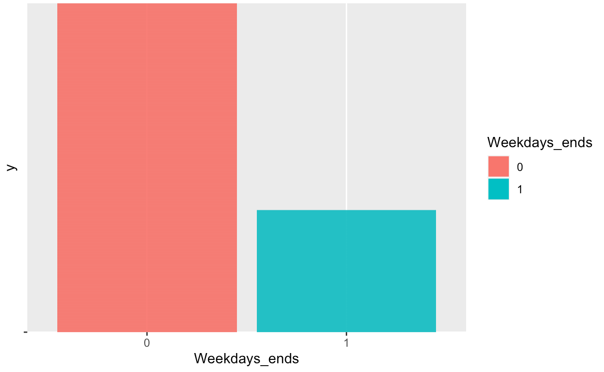
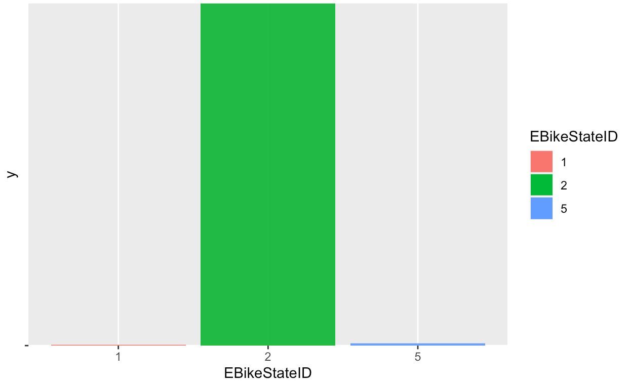
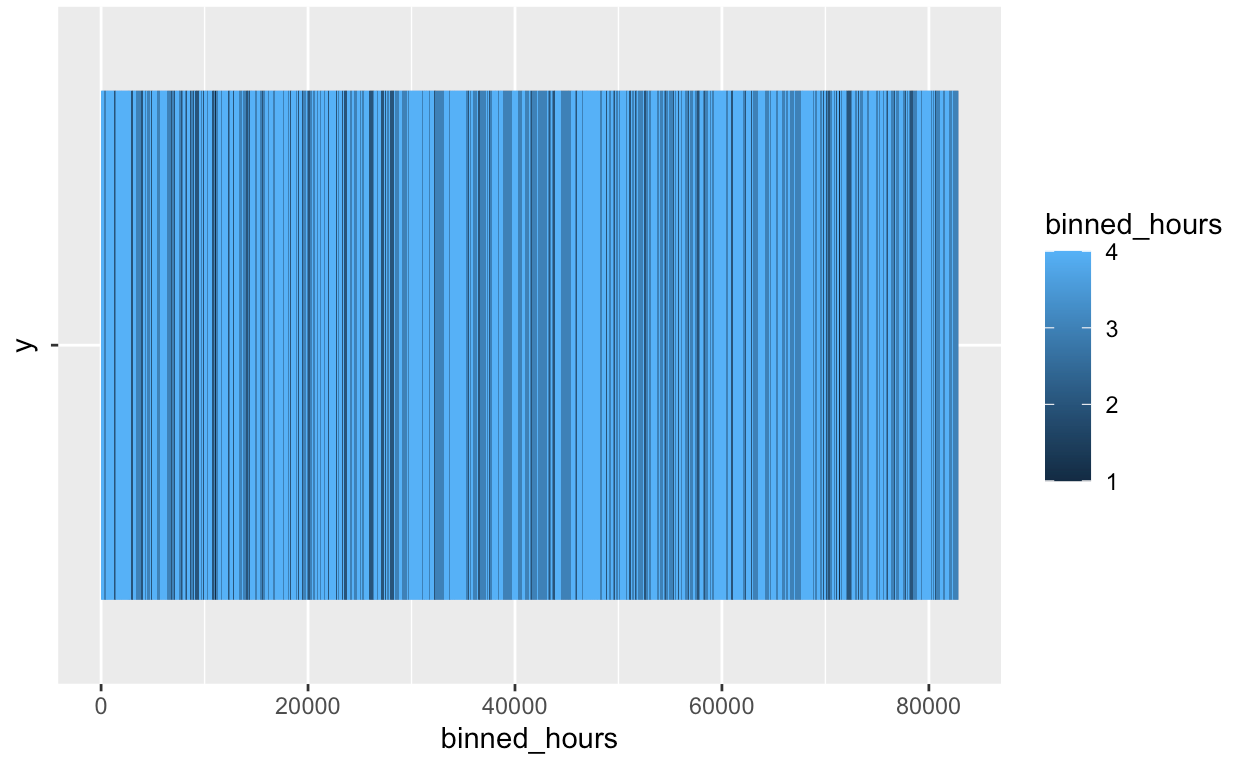
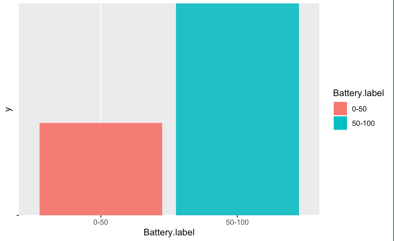
These visualizations give important information about the data. From looking at these graphs,
it can be concluded that our label "Battery. Binned" is not balanced. As such, an oversampling
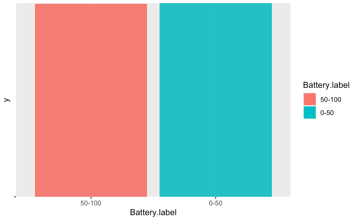
method has been applied on the less frequent "Battery.binned" value. The resutling graphs shows that
The oversampling has now balanced the dataset.

after the data cleaning process, the data set has been divided into a training set and test set. The test set is 3/4 of the entire data set.
Model Building
In the model building section the results of three different Decision trees will be demonstrated.
The Decision Trees differ from eachother because of the tuning to the complexity Parameter .
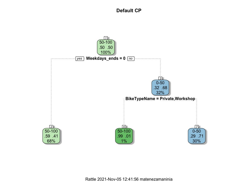
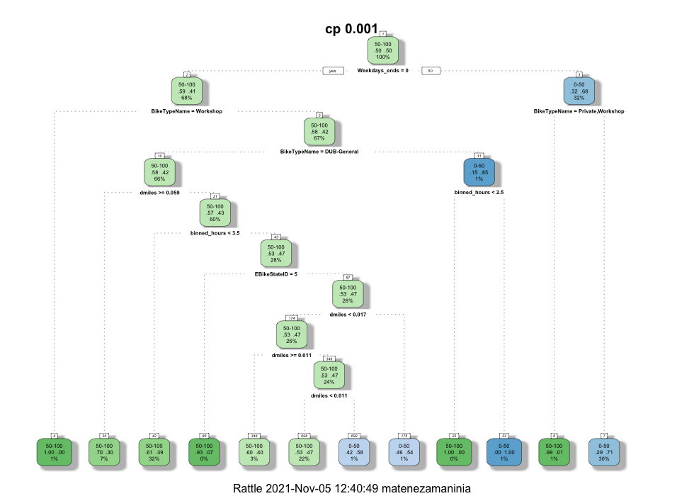
The values of CP appplied to the decision tree are : default = 0.01, 0.005, 0.001. The resulting DecisionTrees can be seen below.
Default CP

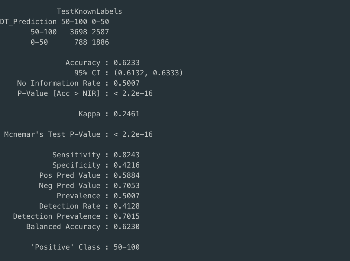
Confusion Matrix

CP = 0.005

Confusion Matrix

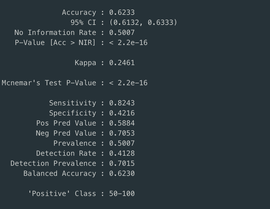
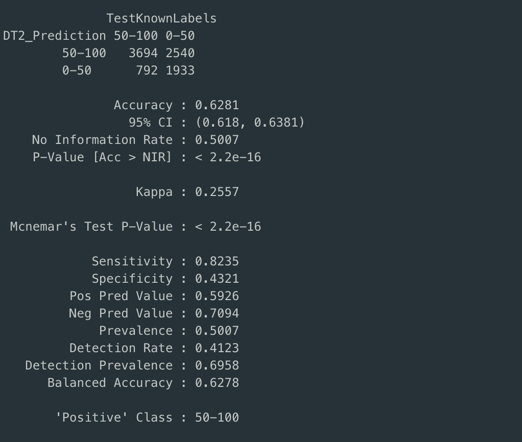
Observe that for both the default value of cp and cp = 0.005, the decision trees are identical.
The accuracy of prediction for both of the decision trees is close to 62%, sensitivity82% and specificity is equal to 42%.
CP = 0.001

Confusion Matrix

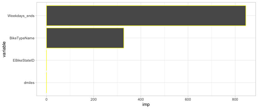
From the Decision trees it can be seen that whether the the day is a weekday or weekend has the most predictive ability.
To see the order of predictive ability, a variable importance plot has been produced.

Clearly, the weekday vs weekend variable and biketype have the most predictive power.
Random Forest
random forests is an ensemble learning method for classification and regression.
It operates by constructing a multidue of decision trees at training time. The random forest algorithm
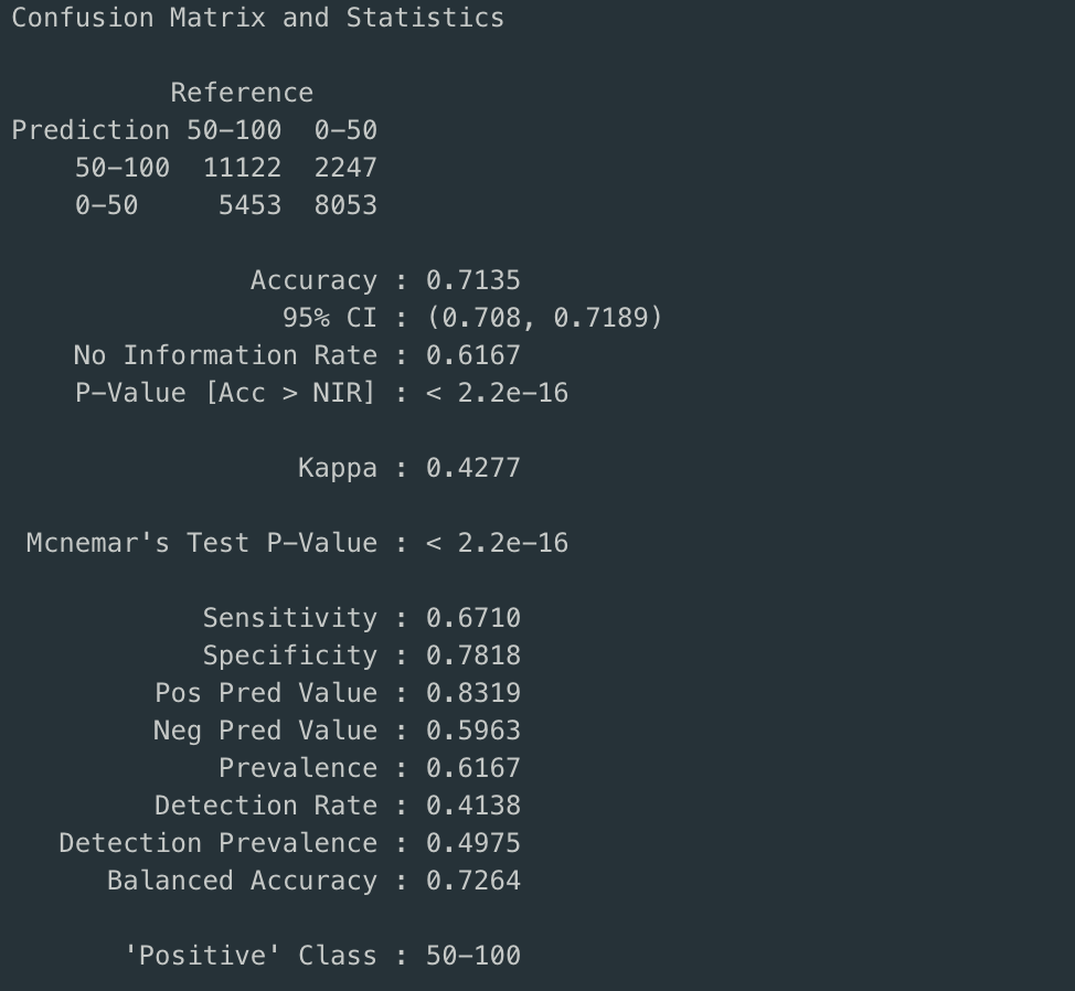
was used on the mentioned dataset. From the confusion matrix below it can be observed that the
random forest has higher accuracy (from 62% to 71%) and specificity(from 0.43 to 0.78) but has less
sensitivity(0.67% from 0.82%). The conclusion from this will be mentioned in the conclusion section.

Additionally, the variable importance plot of the random forest indicates that the miles traveled is more important than whether it is a weekday or weekend.

Decision Tree for Text Data in Python
The code and dataset .

In this section, an implementation of decision tree on text data. Similar to any other method used, the preprocessing step is critical and will be explained first.
Data Cleaning and pre-processing
The data cleaning process for decision tree is similar to the cleaning done for the clustering assignment as opposed to the ARM method.
There is however one simple distinction; The label words are also ommited from the bag of words used.
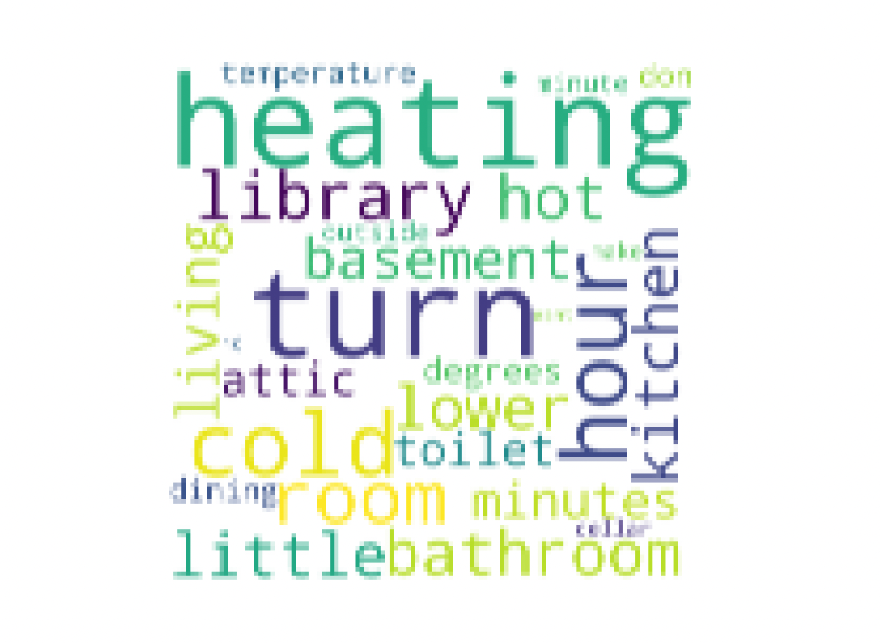
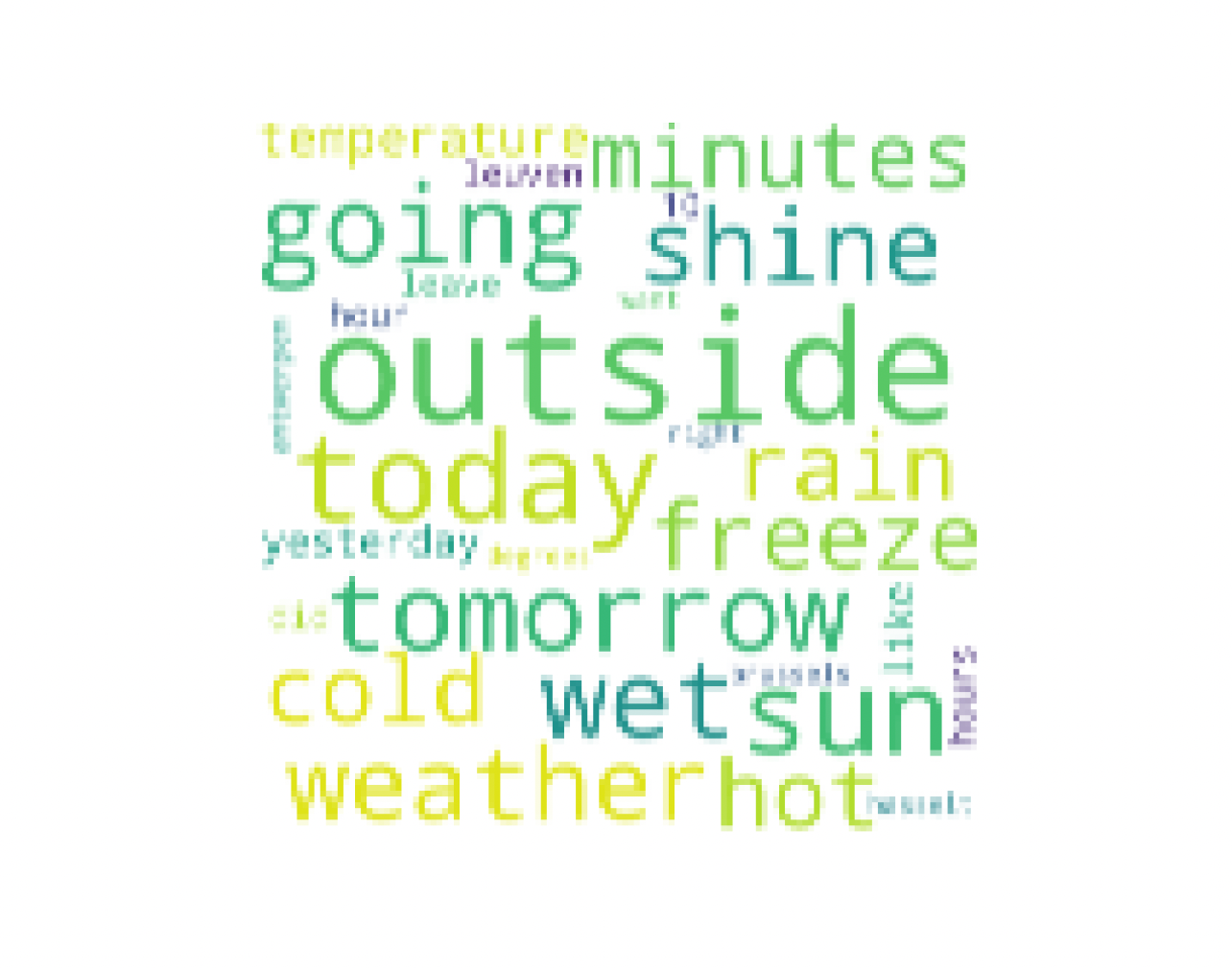
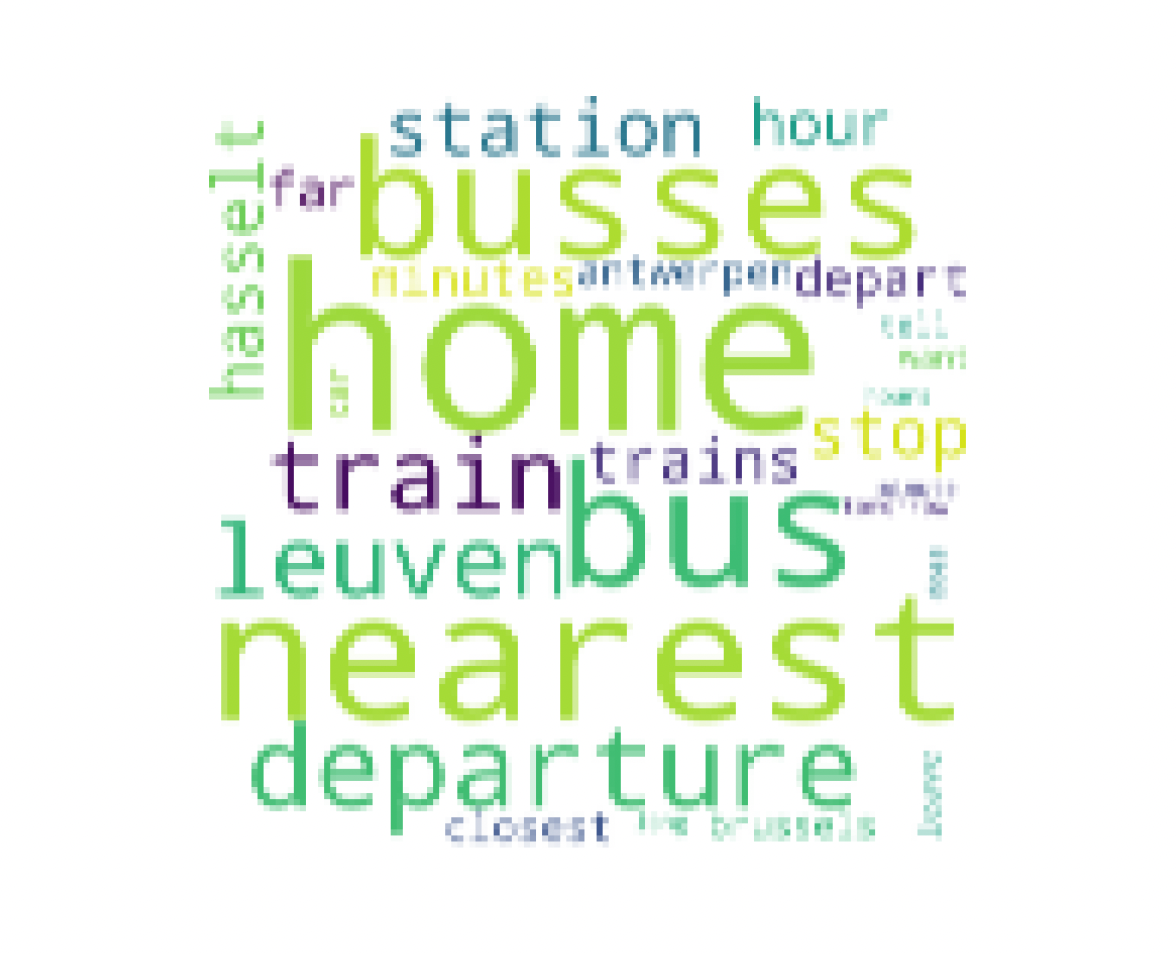
After the data is cleaned and in the desired format, A word cloud was created for each label. A few of them can be seen below.
Heating

Weather

Direction

Model Training and Testing
To perform model building the data set is subsetted to 4 data frames:
1) Test label
2) Test data
3) Training label
4) Training data
After partitioning the data into the subsets, a Decision Tree with our desired parameters is instantiated.
After creating the desired version of a decision tree, the training data and its label are used to create the following decision tree.
Open PDF file example.
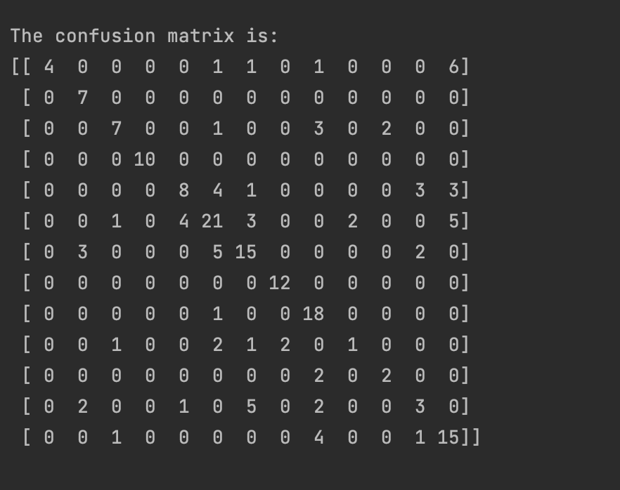
Additionally, The following confusion matrix can give us statistics on how well the model is performing.

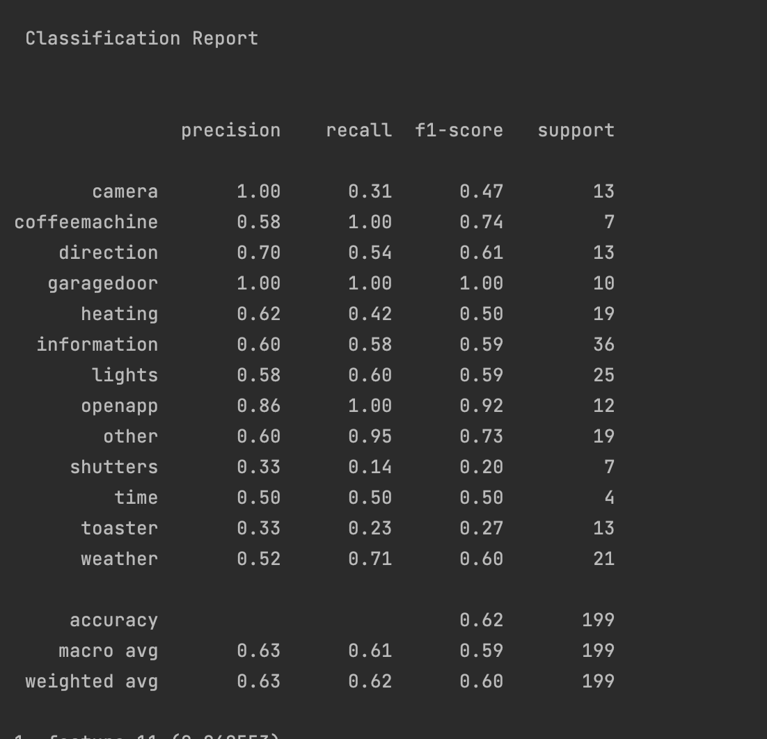
From the matrix we can see that the results are relatively well. Lets get some more absolute statistics on how the model is performing.

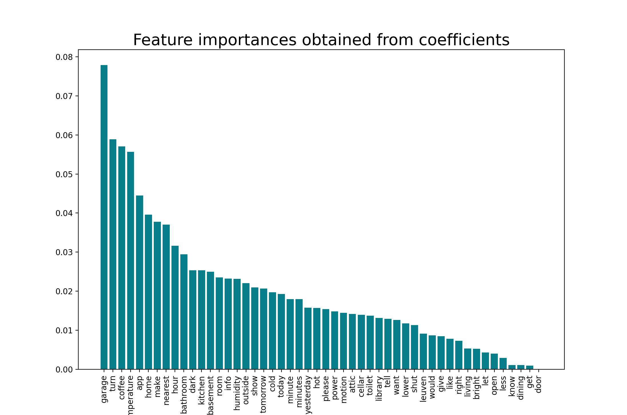
Additionally, the following variable importance plot has been constructed. It shows that the top 5 words
with predictive power are:
"garage", "turn", "coffee", "temperature" and "app".

Conclusion
From this illustration the ability and flexibility of decision trees can be observed.
The record data was ran on "mixed data", this means that the model was able to use
values that come in different forms. For example, the dmiles values are numbers,
while the biketype is a category.
In the previous methods such as clustering and ARM this was not possible.
The model had an accuracy rate of 63%.
In the random forest section the capabilities of ensemble learning was demonstrated.
we saw that the random forest method was able to increase accuracy of prediction
from 63% to 71%. Additionally, the specificity of the model also increased from 0.43 to 0.78.
This means that the models ability to predict battery percentages above 50% increased by 35%.
Additionally it was illustrated that the decision tree is also implementable for Text data and that
the model provided fairly decent results. From the confusion matrix we see that the model has a 62% accuracy
which is impressive.
