Clustering
In this section, applications of clustering will be demnostrated on both text as well as record data:
Perparing Data for Clustering using both
R and Python
Different algorithms and methods have different data requirements that must be met. As such , before model building it must be insured
that the data being used is in the proper format. For our example of clustering on record data the "Moby-Bikes" Data set, shown in the data cleaning section, will be utilized. In addition
to the basic cleaning done in the previous section, additional cleaning and feature generation will be conducted in order to prepare the data for model building. In the Data Cleaning section, after addressing data
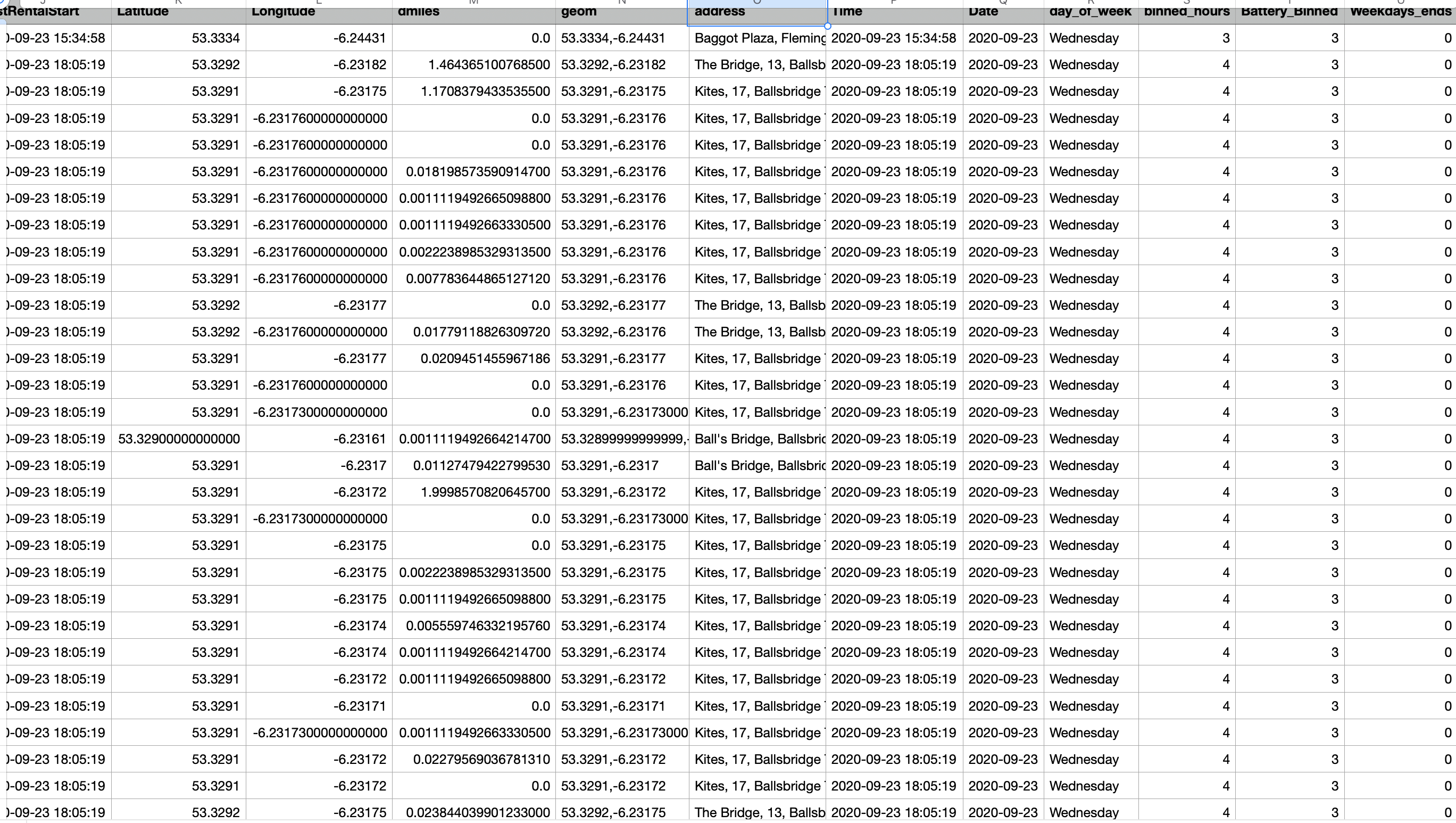
cleaning issues, feature generation was demonstrated by calculating the distance traveled bewteen each time x(t) and x(t-1). The resulting attribute was added as "Dmiles". Further more, the Latidude and Longitude were used to create a second generated attribute which produced the exact address of each bike. In this section a number of new features will be generated. For your conveniance, the
code for that process has been also added here.
The "LastRentalStart" attribute, will be split into two columns: 1) Date 2) time
From the Date attribute, for each row, we obtain a new attribute, "day of week"
From the "day of week" attribute we create two new features. First) a fearture that has the days of the week as numeric
values (Monday = 1, Tuesday = 2 and so on). Second) we create a binary feature of 0s and 1s that specifies if a given day
is a week day or weekend.
From the "day of week" attribute we create two new features. First) a features that has the days of the week as numeric
values (Monday = 1, Tuesday = 2 and so on). Second) we create a binary feature of 0s and 1s that specifies if a given day
is a week day or weekend.
The Longitude and Latitude for each bike at each 30 minute interval were sent to a server and the exact address of the bikes were obtained as
a new feature. (This was added to the code from last weeks data cleaning. The link has been updated since. If planning to run the code, do be cautios as it
takes several hours for the preocess to be
The hours of day were further binned into 4 intervals. (0-6,6-12,12-18,18-24). Each interval was assigned a numeric value.
The Battery levels were also binned into 3 intervals (0-30, 30-60, 60-98).
The dataset can be seen here. The python code is also accessible through this link a snippet of the new features can be seen below.

The resulting data set was imported into R to conduct data transformations and model building. Only a part of the resulting data set will be used in the model building. As such
we subset tyeh follwoing columns from the data set : "Battery", "BikeTypeName", "EBikeStateID", "Latitude", "Longitude", "dmiles", "day_of_week", "binned_hours", "Weekdays_ends".
The "Battery" attribute is the label so it has been further stripped and saved separately. The attributes "BikeTypeName", "EBikeStateID","day_of_week", "binned_hours", "Weekdays_ends" have all been
numericized and then transformed to ordered factors. Other variables are in integer format so they need not be further transformed.
Model Building in R .
Hierarchical Clustering
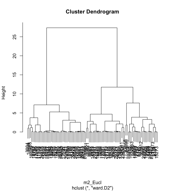
The first example of model building will be demonstrated for hierarchical clustering using three different distances. The first example is the hierarchical clustering using the euclidean distance. The dendogram and distance matrix of which can be seen below.


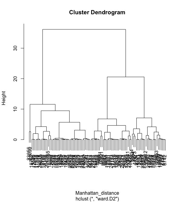
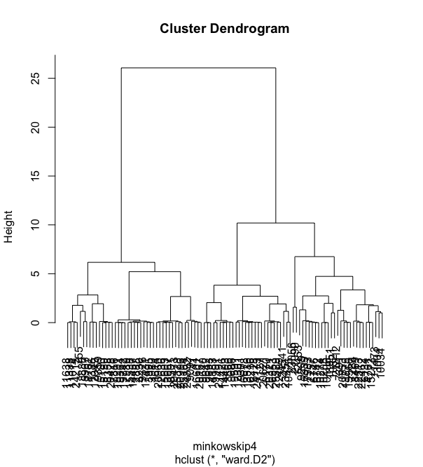
We can see that the hierarchical clustering with euclidean distance does not generate clear clusters. The two graphs below are hierarchical clustering with Manhattan distance and also miknowski distance with p = 4.


We can see that although the graphs are different, none of them really are able to create good clusters.
However, we can see that there seems to be 4 Main clusters!
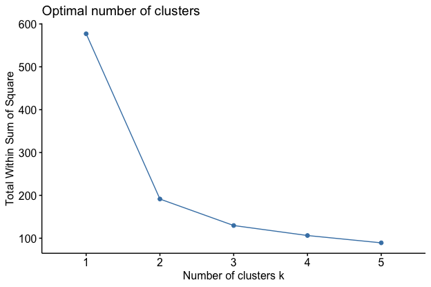
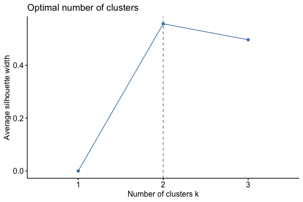
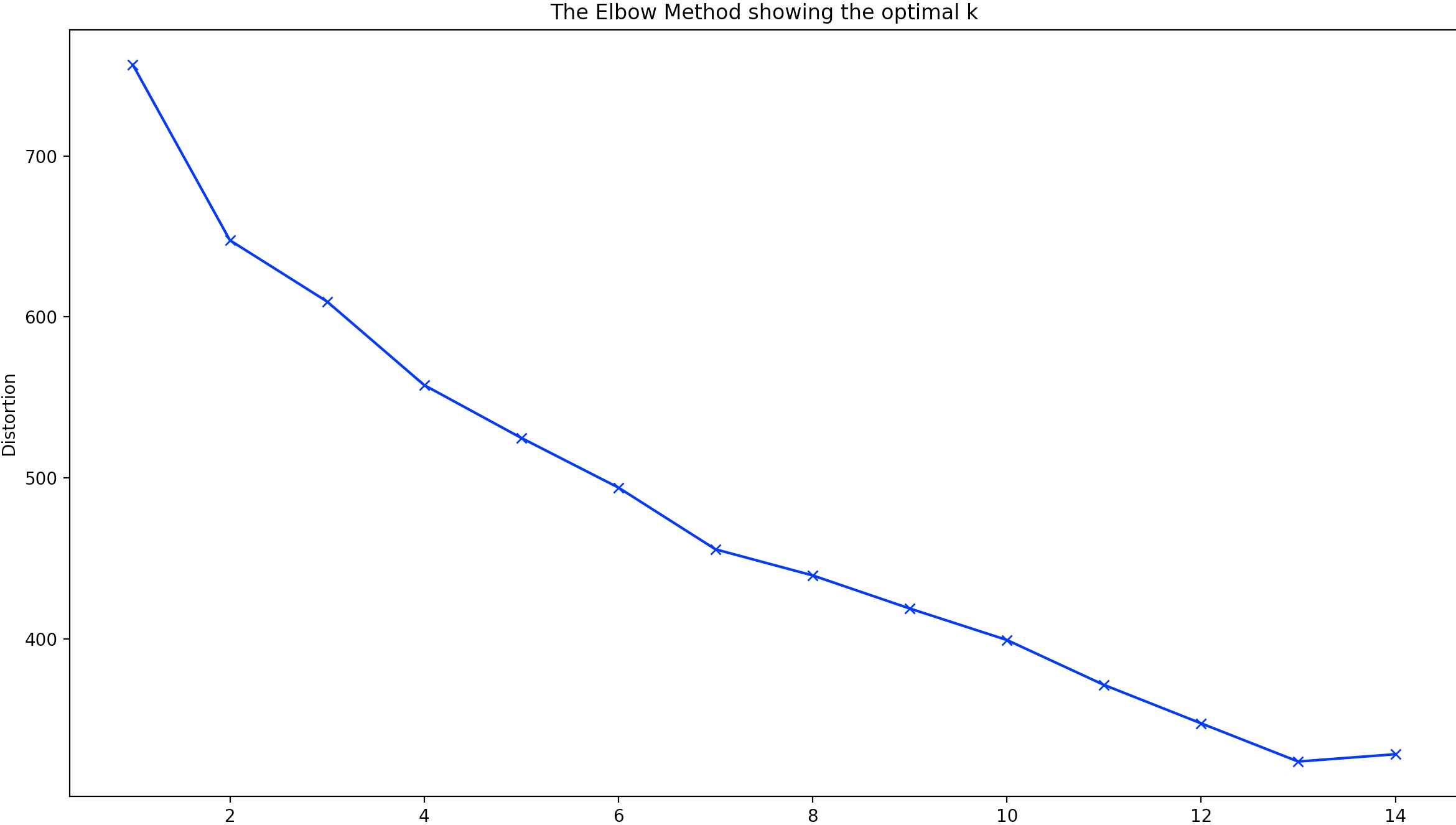
To verify this we use a elbow plot and a Silhouette plot to help in identifying the best number of cluseters.
Elbow plot

Silhouette plot

We can see that both agree that the best K = 2
Text Data Clustering
For the text data, in order to create less confusion, the entire code of the analysis from cleaning to modeling and
graphing has been done in a single section which utilizes the original data set data set
Analysis
As a reminder, the data set contains information about commands given to smart home devices and how they are related to different aspects of a house. The objective of this part of the analysis is to find whether we can group these
commands(words) to pertain to the correct part of the house.
After the initial data cleaning process, the labels were removed and saved in a seperate dataframe. It is known that the original
dataset contains 13 different categories of labels which are:
lights,camera, open app, direction, information, other, weather, heating, shutters, toaster, garagedoor, coffeemachine and time.
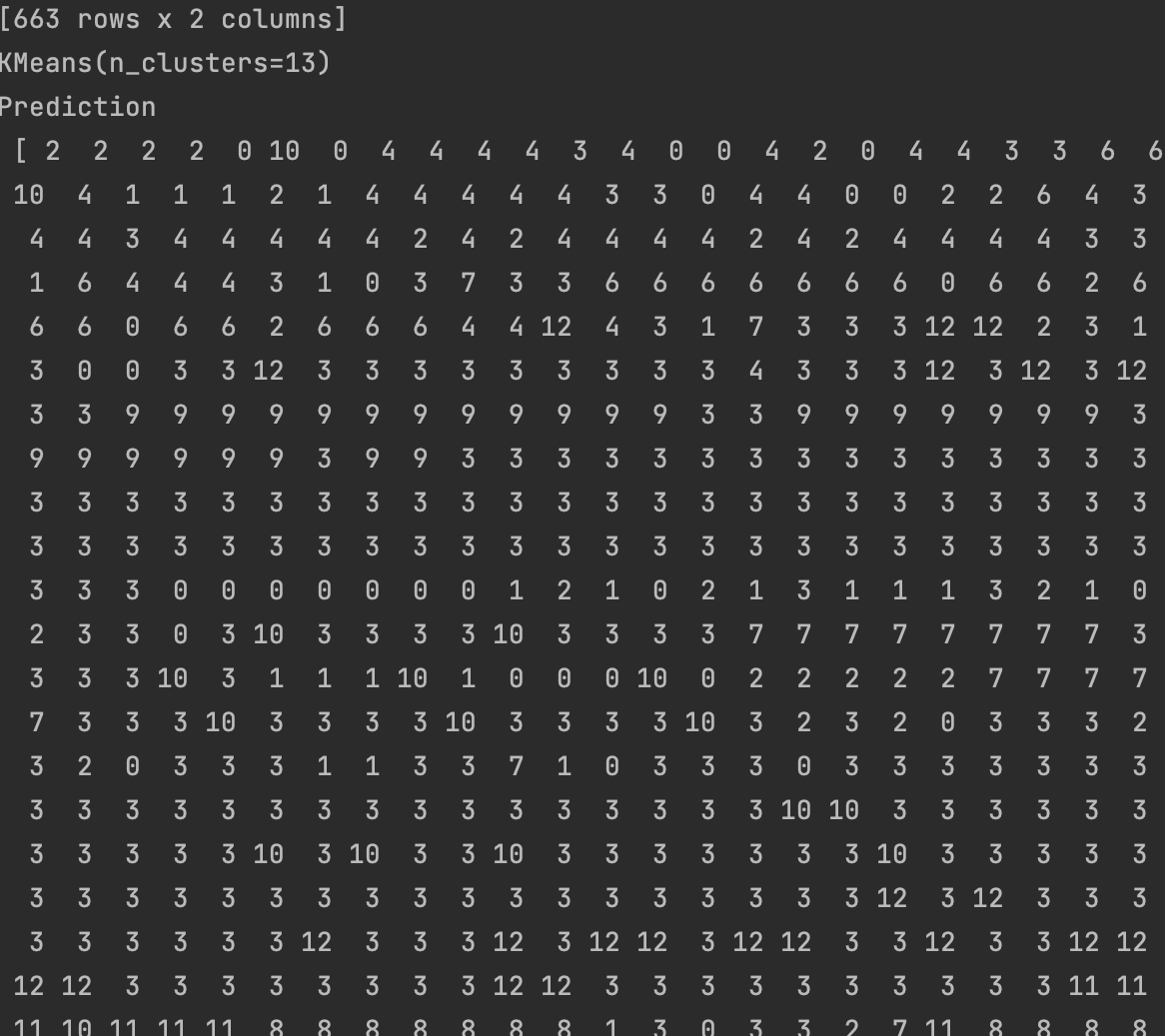
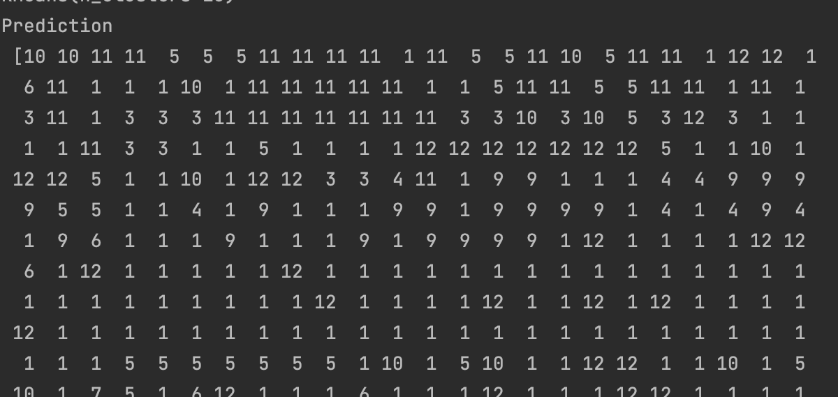
Three different values of K was used for the analysis to compare the results. The K values are: k = 13, k= 10 and k = 17.
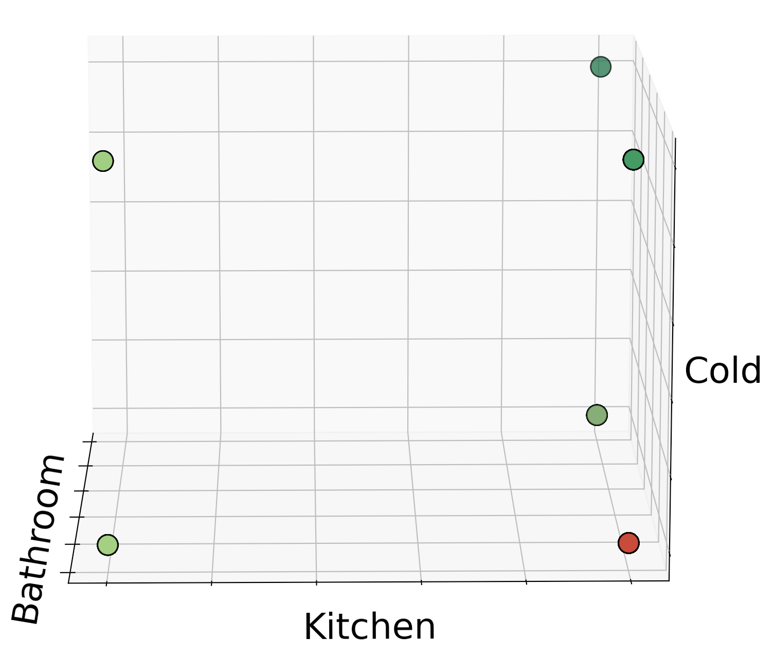
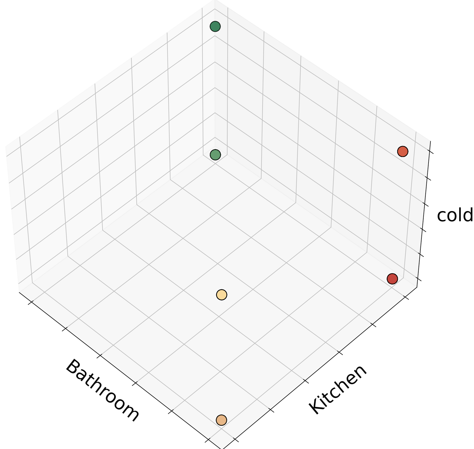
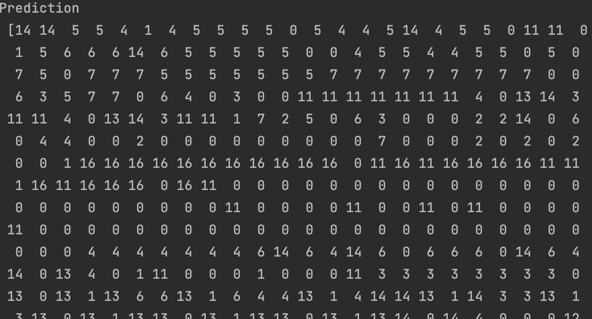
The result of the analysis is brought below. for better understanding the label of the data is shown next to the models prediction. For each model, a 3D graph of the same 3 words are also
shown for better comprehension. Keep in midnd, two labels should not be labeled with different predictions, but we can see that this is often the case.
K = 13

K = 10


K = 17


It is obvious that the rows have been assigned incorrectly, but difference values of k have created different issues.
NETID : MZ569
PCA
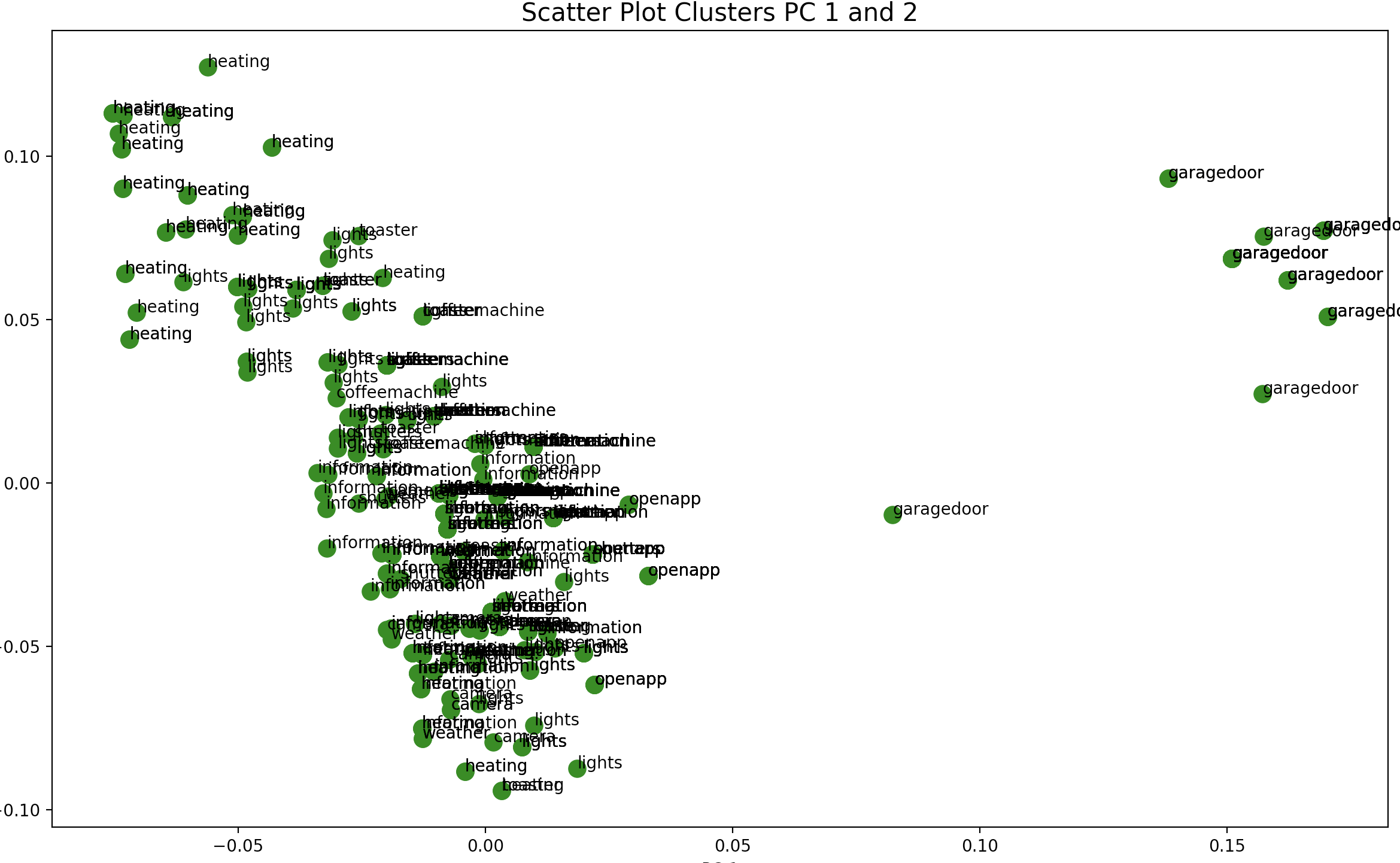
Because of the high dimensionality of the data a Principle Component Analysis was conducted to assist in better
understanding of our results. From the PCA, the follwoing results were extracted.

This graph is interesting in that it shows the PCA determined the garagedoor to be a completely seperate cluster. An interesting continuation
of this analysis would be to remove the garagedoor label and to see if the PCA is able find other distinct groups.
DBSCAN
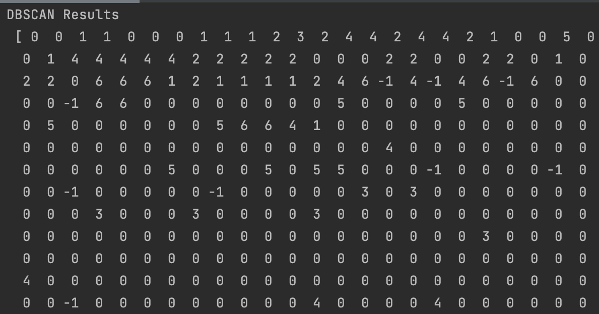
The DBSCAN was ran on the components of the PCA. The results did not reveal an ability to distinguish between clusters correctly.

Hierarchical Clustering
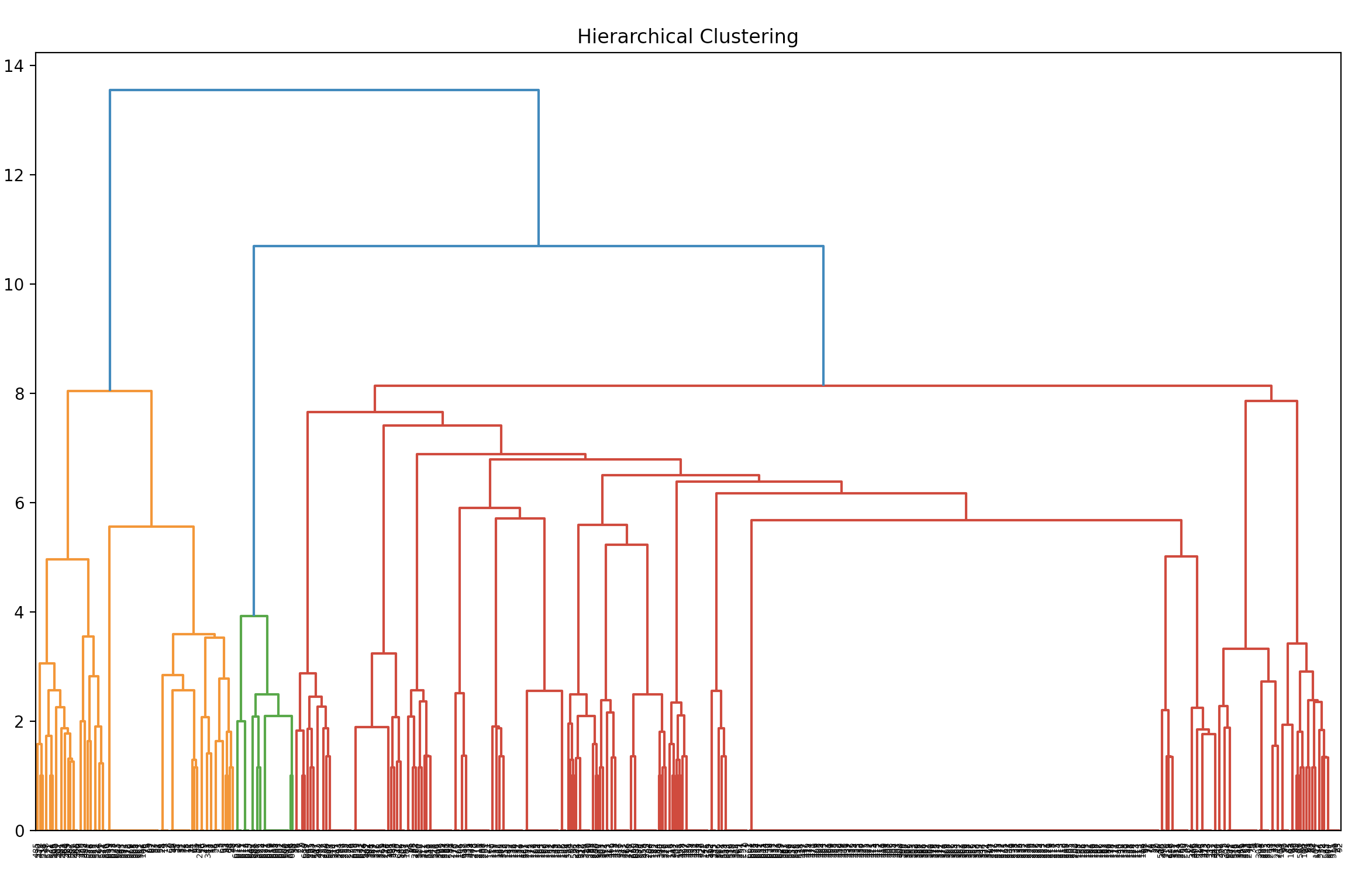
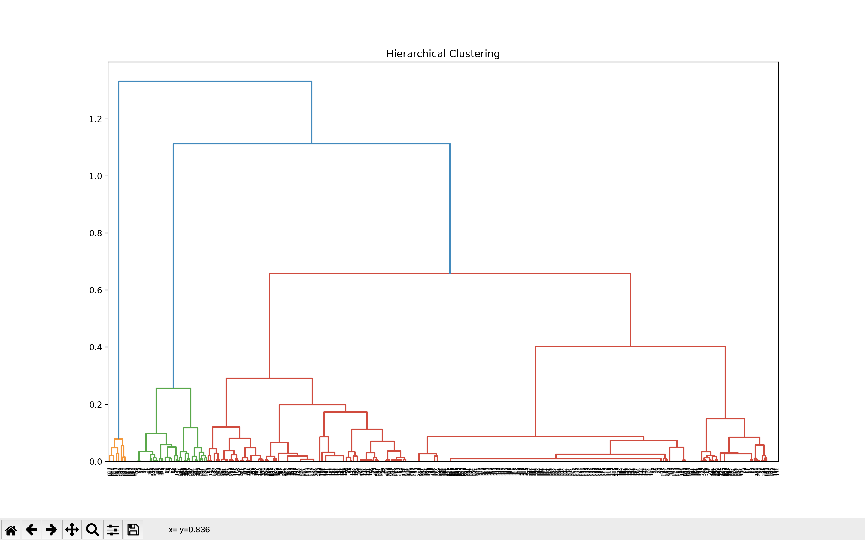
The Hierearchical Clustering algorithm was ran on both the PCA results as well as the normal results. While the result of the PCA is much clearer, It is still unable to correctly identify the
data clusters.
Regular Dendogram :

PCA Dendogram :

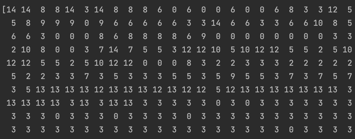
The results of the PCA class labels is also brought below:

Again, it can be observed that even though the algorithm worked, there are many mistakes in the predictions.
As part of the analysis an elbow plot was also constructed to see the different values of predicitons made by the algorithm.

conclusion
We can see from the text analysis that the algorithms did not perform well on the data. This could be due to the data being unsusceptiblity to this type of algorithms.
